|
SECTION 5
SPATIAL DECISION SUPPORT
Section 5 - Site selection - Locational analysis and location/allocation - Other forms of operations research in spatial analysis - Spatial decision support systems - Linking spatial analysis with GIS to support spatial decision-making:
- Shortest path, traveling salesman, traffic assignment.
- What is location/allocation, and where can it be applied?
- Modeling the process of retail site selection. Criteria.
- Electoral districting and sales territories.
- What is an SDSS? What are its component parts? How does it compare to a GIS or a DSS? Why would you want one? Building SDSS.
- Examples of SDSS use - site selection, districting.
Methods of analysis on networks
A spatial database can be used to support the solution of a variety of network problems, including optimal location, routing and vehicle scheduling
Routing:
Shortest path problem
Traveling salesman problem and variants
Trans-shipment problem
Hitchcock transportation problem
Traffic assignment problem
Location:
- solution of many of these problems raises a number of issues of data modeling
-
- some of these have been raised earlier in the example of modeling a street network for shortest path analysis
-
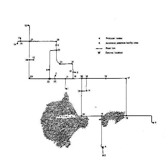
Example: Brine disposal in the Petrolia, Ontario oil field
- oil extraction from the field generates large quantities of waste fluid
- there are 14 active producers in the field, each operating a single extraction facility
- the only effective method of disposal is by pumping to a formation below the oil producing layer
- options include:
-
- a single, central disposal facility
- requiring each producer to install a facility
- some intermediate configuration of shared facilities
One disposal well per producer:
One central facility:
The location-allocation problem:
- find locations for one or more central facilities and allocate producers to them in order to minimize the total of capital and transport costs
-
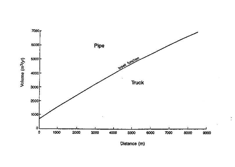
Two alternatives for transport of waste brine to central facilities: pipe and truck.
Pipe cost:
C1 = A D0 / B + C
A installed cost per metre
D0 distance in metres
B pipe life in years
C pump cost per year
Truck cost:
C2 = E D V0 / (365 F) + Q V0 (H + D0/(1000P)) / G
E holding period, days
D holding capacity, m3
V0 volume of brine, m3 per year
F life of holding capacity, years
Q truck cost, $/hour
H time to load and unload truck
P speed of truck in km/hour
G truck load, m3
Disposal well cost:
New well - $50-$75,000
Success rate 60-80%
Buildup of residual hydrocarbons
Corrosion of pipes
Slide: Petrolia area
Slide: Transport cost functions
GIS implementation:
Network of streets and rights of way - potential routes for trucks/pipes
Links with attributes of length
Nodes with attributes of volume produced - producer sites plus other potential well locations
GIS database with nodes and links and associated attributes:
- data input functions (editing)
- data display - graphics, plots
- storage of geographic data
- provides data to the analysis module
-
Analysis module interacting with GIS database
- obtains nodes and links from the GIS
- performs analysis, reports results directly to the user
- includes several heuristic methods for solving the optimization problem
- allows the user access to the display/analysis functions of the GIS
-
An analysis module supported by a GIS database provides a spatial decision support system (SDSS) tailored to specific, advanced forms of spatial analysis
Location-allocation analysis module:
1. Finds shortest paths between points on network (could be a GIS function)
2. Define and modify model parameters
3. Use paths and parameters to calculate transport costs
4. Search for optimum solution using add, drop and swap heuristics
5. Evaluate solutions and print results
| Option |
Number
|
Facility cost
|
Transport cost
|
$/m3 brine
|
$/m3 oil
|
| All producers |
14
|
165,000
|
0
|
1.32
|
26.42
|
| Central by truck |
2
|
45,000
|
395,827
|
3.53
|
70.59
|
| Central any nodes |
2
|
60,000
|
79,619
|
1.12
|
22.36
|
| Central any producers |
2
|
60,000
|
80,658
|
1.13
|
22.52
|
| Existing disposal wells |
2
|
30,000
|
92,031
|
0.98
|
19.54
|
| Parameter |
Value
|
% pipe
|
% truck
|
Optimum sites
|
Cost $000s
|
| Pipe cost A |
30
|
74
|
26
|
4,8
|
80.7
|
| |
60
|
53
|
47
|
2,4,7,9
|
76.3
|
| |
15
|
87
|
13
|
4,8
|
56.6
|
| Pipe life B |
10
|
74
|
26
|
4,8
|
80.7
|
| |
8
|
67
|
33
|
2,4,7
|
73.0
|
| |
6
|
62
|
38
|
2,4,7,9
|
69.4
|
| |
4
|
47
|
53
|
2,4,7,9
|
86.0
|
| Pump cost C |
2000
|
74
|
26
|
4,8
|
80.7
|
| |
1000
|
77
|
23
|
2,4,7
|
52.8
|
| |
500
|
77
|
23
|
2,4,7
|
46.8
|
| Well cost R |
60,000
|
74
|
26
|
4,8
|
80.7
|
| |
100,000
|
74
|
26
|
4,8
|
80.7
|
| |
40,000
|
74
|
26
|
2,4,7,9
|
54.6
|
| Life of well S |
4
|
74
|
26
|
4,8
|
80.7
|
| |
8
|
74
|
26
|
2,4,7,9
|
54.6
|
| Brine ratio U |
25
|
74
|
26
|
4,8
|
80.7
|
| |
30
|
82
|
18
|
2,4,7
|
69.0
|
| |
40
|
90
|
10
|
2,4,7,9
|
59.8
|
| |
60
|
96
|
4
|
2,4,7
|
70.1
|
Other examples of complex GIS-based analysis:
Vehicle routing and scheduling
Traffic modeling
Corridor location for pipelines/powerlines/highways
Runoff modeling based on DEM
Load balancing in electrical networks
Spatial search
Boolean search
Search through an attribute table to find objects satisfying a set of criteria
Example:
Forest stands - area object type, non-overlapping
Attributes: area (reserved)
For each stand, compare species and age to desired criteria.
Dissolve and merge boundaries between neighboring stands if both fit the criteria
Use tables to obtain estimated yield for given species/age and area
Generate a map showing merged groups of cuttable stands, with new IDs, plus a table showing yield for each group.
Topological overlay
Two or more coverages can be overlayed to obtain new object types with concatenated attributes. This allows Boolean search and related operations to be conducted on multiple object types, i.e. with more information available.
Example:
Add soil moisture information, from a separate coverage, to the criteria used to identify cuttable stands.
Buffer zone generation
A buffer zone allows Boolean searches to include criteria based on distance
Example:
A stand is cuttable only if it is not less than 200m from the nearest stream/lake
In many cases it is not possible to reduce all criteria to simple yes/no requirements.
e.g. from those stands satisfying criteria 1 and 2, select that stand which minimizes total cost (sum of criteria 3, 4 and 5)
When all non-conditional criteria are commensurate (dollars) they can be summed.
In many cases criteria are not commensurate and cannot be summed.
Example
1. Timber extraction/hauling costs - direct $ costs
2. Environmental cost of extraction - intangible
3. Road construction cost - $, but long-term benefits
Decision Theory provides methods for determining:
Single Utility Functions (SUFs) for each criterion
Multiple Utility Functions (MUFs) to combine criteria.
Both SUFs and MUFs can be determined by experimental designs involving groups of decision-makers
Decision theoretic methods can be incorporated into GIS technology. The GIS is used to evaluate the criteria for each alternative, then to weigh them using SUFs and MUFs to arrive at a decision.
A model for spatial analysis with a GIS
Example of multi-stage GIS analysis
Generation of a Recreation Opportunity Spectrum (ROS) map for a National Forest 1:24,000 quad (7.5 minute)
Problem: generate zones and associated ROS classes for Forest Service land based on distance from transportation features, with urban exclusions.
Data needed:
D1: Roads and railways (1:24,000) - line objects
D2: Forest Service ownership map (1:24,000) - area objects
D3: City and town boundaries map (1:24,000) - area objects
GIS functions:
Reclassify attributes (B2)
Dissolve and merge (B3)
Generate corridors (B24)
Topological overlay (B50)
Measure size of areas (B35)
Centroid calculation and sequential numbering (B8)
Plot (A12)
Create list and report (B1)
Steps to make product:
1. Using the forest service ownership data, reclassify area objects as forest land / not forest land. (B2)
2. Dissolve boundaries between polygons with the same value of the forest land / not forest land attribute, and merge polygons (B3)
3. Using the transportation map, generate corridors 0.5 miles wide around all roads and railways. (B24)
4. Using the transportation map, generate corridors 1.0 miles wide around all roads and railways. (B24)
5. Topologically overlay the results of 2, 3 and 4 and concatenate the attributes, to obtain polygons with the following attributes:
forest land / not forest land
within/outside 0.5 mile corridor
within/outside 1.0 mile corridor (B50)
6. Topologically overlay the urban boundary map, and concatenate attributes, adding urban/non-urban to the list in 5. (B50)
7. Reclassify the area objects resulting from 6 according to the following rules:
Class Criteria
Null not forest land
RMU forest land and urban
SPM forest land, non-urban and within 0.5 miles of road/rail
SPN forest land, non-urban, outside 0.5 mile and inside 1.0 mile corridors
P forest land, non-urban, outside both 0.5 mile and 1.0 mile corridors (B2)
8. Dissolve and merge adjacent polygons with the same class (B3)
9. Measure areas of polygons resulting from 8 (B35)
10. Reclassify polygons of class SPM according to the following rules:
SPM Areas of less than 2500 acres
RN Areas of more than 2500 acres (B2)
11. Calculate centroids and sequentially number polygons (B8)
12. Plot classified polygons with classes and numbers assigned in 11, plus roads and railways and urban areas (A12)
13. Create a list of all polygons, with IDs, areas and classes. (B1)
Summary sequence of operations:
Initial data sets: D1, D2, D3
1. B2 on D2 -> E1
2. B3 on E1 -> E2
3. B24 on D1 -> E3
4. B24 on D1 -> E4
5. B50 on E2, E3, E4 -> E5
6. B50 on E5, D3 -> E6
7. B2 on E6 -> E7
8. B3 on E7 -> E8
9. B35 on E8 -> E9
10. B2 on E9 -> E10
11. B8 on E10 -> E11
12. A12 on E11, D1, D3
13. B1 on E11
Many GIS applications require complex decision rules in reclassification operations.
e.g. finding the most cuttable stand of timber:
Criterion
1. Area of stand > 100 acres (B35)
2. More than 100m from stream/lake (B24)
3. Subrules based on slope, aspect and soil mechanics determine method of timber extraction.
4. Analysis of existing roads and terrain leads to estimates of costs of constructing new
roads and hauling timber to mill
5. Subrules based on costs of replanting, silviculture
Districting
- GIS technology useful in designing sales areas, analyzing trade areas of stores
- similar applications occur in politics
-
- design of voting districts (apportionment, gerrymandering) has enormous impact on outcome of elections
- major interest in reapportionment after 1990 census
- GIS applications in these areas are still at early stage
Characteristics of application area
- scale:
-
- street centerline, census reporting zones - i.e. 1:24,000 and smaller
- data at block group/enumeration district scale (250 households) is needed for locating smaller commercial operations like gas stations and convenience stores
- data at census tract scale (2,000 households) is good for the location of larger facilities like supermarkets and fast food outlets
- data sources:
-
- much reliance on existing sources of digital data
-
- especially TIGER and DIME
- similar data available in other countries
- additional data added to standard datasets by vendors
- e.g. updating TIGER files by digitizing new roads, correcting errors
- e.g. adding ZIP code boundaries, locations of existing retailers
- functionality:
-
- dissolve and merge operations, e.g. to build voting districts out of small building blocks
- modeling, e.g. to predict consumer choices, future population growth
- overlay operations, e.g. to estimate populations of user-defined districts, correlate ZIP codes with census zones
- point in polygon operations, e.g. to identify census zone containing customer's residence
- mapping, particularly choropleth and point maps of consumers
- geocoding, address matching
- data quality:
-
- more concern with accuracy of statistics, e.g. population counts, than accuracy of locations
Types of applications
- districting
-
- designing districts for sales territories, voting
- objective is to group areas so that they have a given set of characteristics
- "geographical spreadsheets" allow interactive grouping and analysis of characteristics
-
- e.g. Geospreadsheet program from GDT
- site selection
-
- evaluating potential locations summarizing demographic characteristics in the vicinity
-
- e.g. tabulating populations within 1 km rings
- searching for locations that meet a threshold set of criteria
-
- e.g. a minimum number of people in the appropriate age group are within trading distance
- market penetration analysis
-
- analyzing customer profiles by identifying characteristics of neighborhoods within which customers live
- targeting
-
- identifying areas with appropriate demographic characteristics for marketing, political campaigns
Organizations
- many data vendors and consulting companies active in the field, many large retailers
- no organization unique to the field
- American Demographics is influential magazine
-
Districting example
- GIS has applications in design of electoral districts, sales territories, school districts
- each area of application has its own objectives, goals
- this example looks at designing school districts
Background
- the Catholic school system of London, Ontario, Canada provides elementary schools for Kindergarten through Grade 8 to a city of approx. 250,000
-
- about 25% of school children attend the Catholic system
- 27 elementary schools were open prior to the study
- population data is available for polling subdivisions from taxation records
-
- approx. 700 polling subdivisions have average population of 350 each
- forecasts of school age populations are available for 5, 10, 15 years from the base year at the polling subdivision level
- children are bussed to school if their home location is more than 2 miles away, or if the walking route to school involves significant traffic hazard
Objectives
- minimal changes to the existing system of school districts
- minimal distances between home and school, and minimal need for bussing
- long-term stability in school district boundaries
- preservation of the concepts of community and parish - if possible a school should serve an identifiable community, or be associated with a parish church
- maintenance of a viable minimal enrollment level in each school, defined as 75% of school capacity and > 200 enrollment
Technical requirements
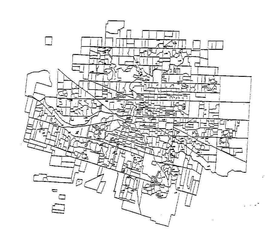
- digitized boundaries of the polling subdivision "building blocks"
- an attribute file of building blocks giving current and forecast enrollment data
-
- for forecasting, we must include developable tracts of land outside the current city limits, plus potential "infill" sites within the limits
- 748 polygons
- development tracts are isolated areas outside the contiguous polling subdivisions
- infill sites are shown as points
- the ability to merge building blocks and dissolve boundaries to create school districts
-
- school districts are not required to be conterminous
- if necessary a school can serve several unconnected subdistricts
- a table indicating whether walking or bussing is required for each building-block/school combination
Slide: City and development areas
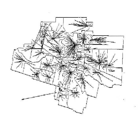
Current districts
- "starbursts" show allocations of building blocks to 29 current schools (includes two special education centers)
-
- note bussed areas in NW and SW - separate enclaves of recent high-density housing allocated to distant schools
- this strategy allows an expanding city to deal with
-
- dropping school populations in the core leading to an excess of capacity
- rising school populations in the periphery but lack of funds for new school construction
- without constantly adjusting boundaries
-
Slide: Current districts
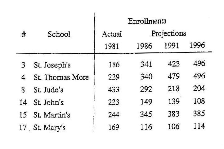
Projections of enrollment based on current school districts
- rapid increase in developing areas, e.g. St Joseph's (#3), St Thomas More (#4) NW
- decrease in maturing areas of periphery, e.g. St Jude's (#8) - SW area
- rejuvenation in some inner-city schools due to infilling, e.g. St Martin's (#15) - lower center
- stagnation in other inner-city schools, e.g. St Mary's (#17), decline e.g. St John's (#14) - center
Redistricting
- general strategy - begin with current allocations, shift building blocks between districts in order to satisfy objectives
- requires interaction between graphic display and tabular output
-
- quick response to "what if this block is reassigned to the school over here?"
- implementation allowed School Board members to make changes during meetings, observe results immediately
-
- using map on digitizer tablet, tables on adjacent screen
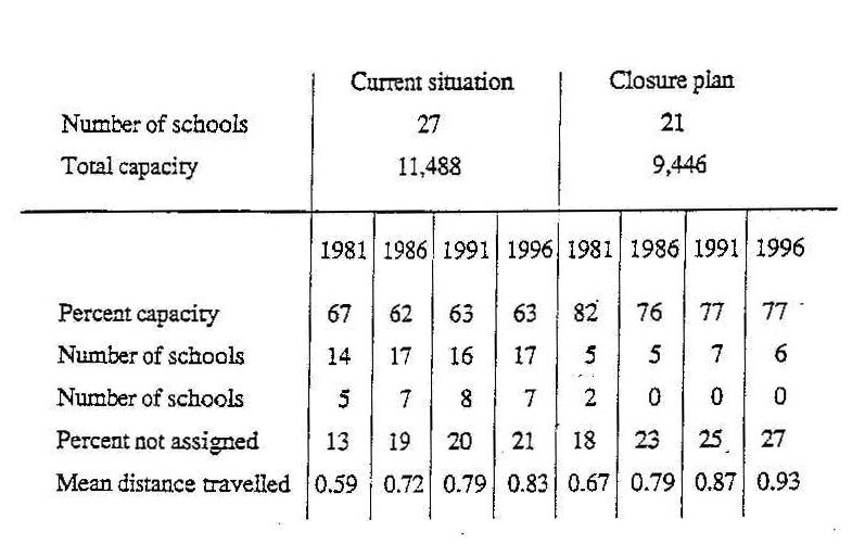
Proposals
- one of the alternative plans developed
- note:
-
- assumes closure of 6 schools
- rise in enrollment as percent of capacity
- stability of projections through time
- reduction in number of "non-viable" schools (<200 enrollment)
- increase in percent not assigned to nearest school
- increase in average distance traveled
Slide: Projected enrolments
Slide: Planned enrolments
|