|
WHAT IS SPATIAL ANALYSIS? Section 1 - What is spatial analysis? - Basic GIS concepts for spatial analysis - GIS functionality - Integrating GIS and spatial analysis - Issues of error and uncertainty:
A set of techniques for analyzing spatial data
"A set of techniques whose results are dependent on the locations of the objects being analyzed"
Some books on spatial analysis:
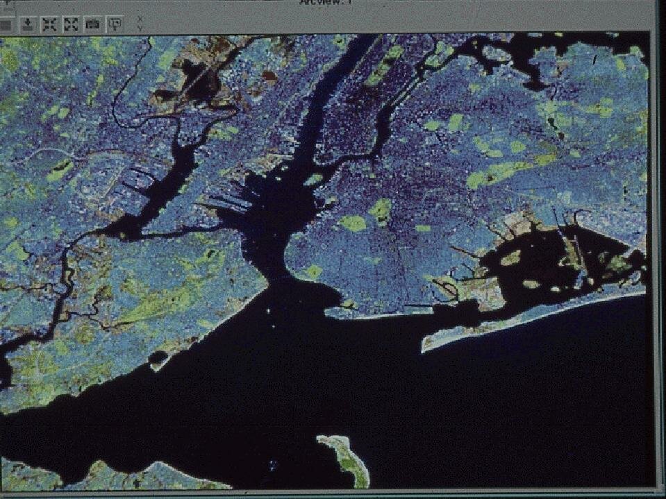
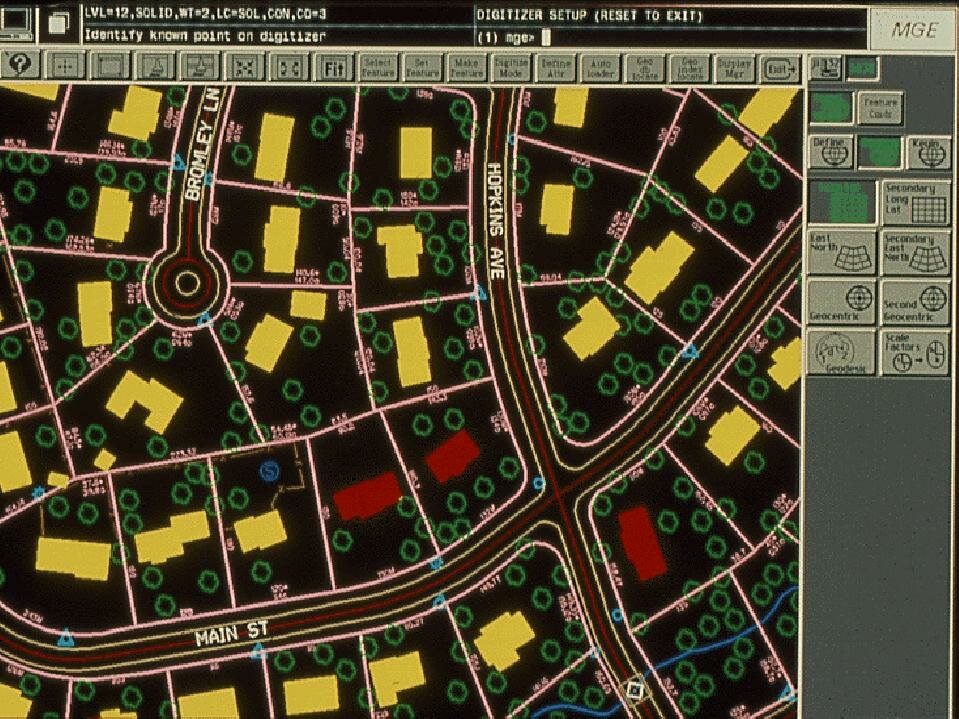
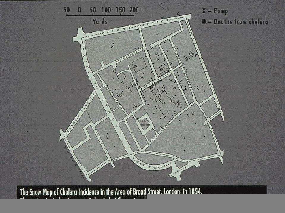
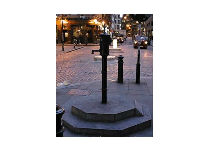
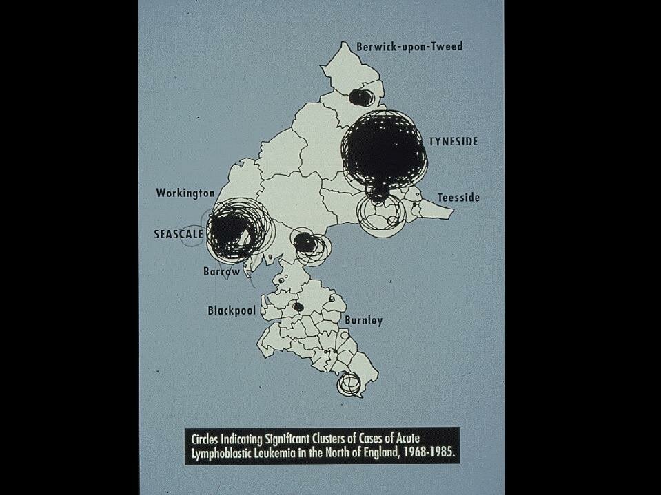
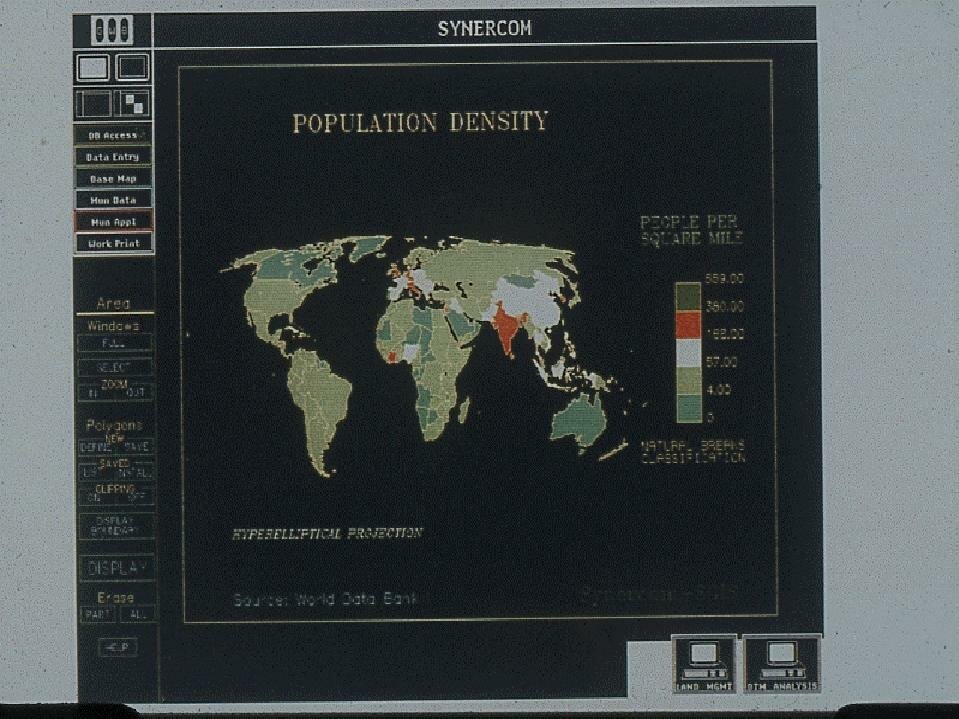
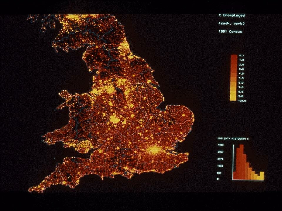
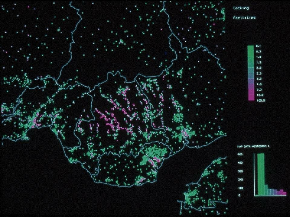
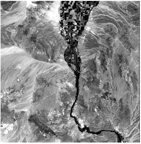
Paul Longley, Mike Goodchild, David Maguire, and David RhindSome background slides: Landsat image of New York areaHow does an analyst/modeler/decision-maker work with a GIS?the pumpOpenshaw GAM map of NE England What tools exist for helping/conceptualizing/problem-solving? Assumption: these (analysis, modeling, decision-making) are the primary purposes of GIS technology. The cost of input to a GIS is high, and can only be justified by the benefits of analysis/modeling/decision-making performed with the data.
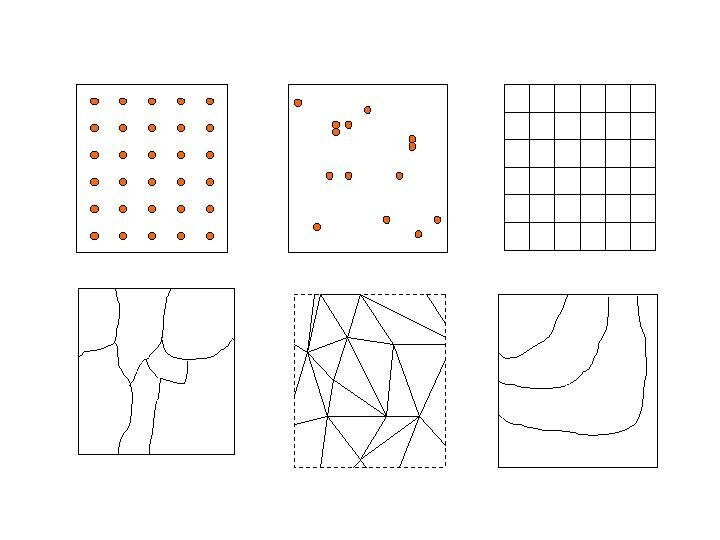
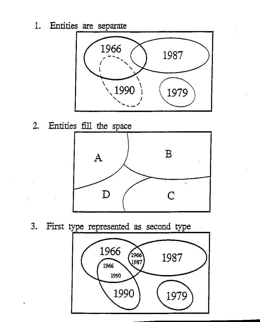
A geographical data model consists of the set of entities and relationships used to create a represention of the geographical world. The choices made when the world is modeled determine how the database is structured, and what kinds of analysis can be done with it. These choices occur when the data are captured in the field, recorded, mapped, digitized, and processed. There are two distinct ways of conceiving of the geographical world. In the field view, the world is conceived as a finite set of variables, each having a single value at every point on the Earth's surface (or every point in a three-dimensional space; or a four-dimensional space if time is included).
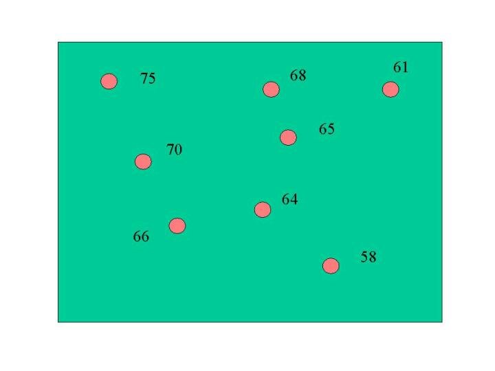
Examples of fields: elevation, temperature, soil type, vegetation cover type, land ownership
To be represented digitally, a field must be constructed out of primitive one, two, three, or four-dimensional objects. There are six ways of representing fields in common use in GIS:
Some field-like phenomena: elevation, spectral response
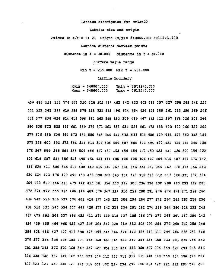
raster (a rectangular array of homogeneous cells)
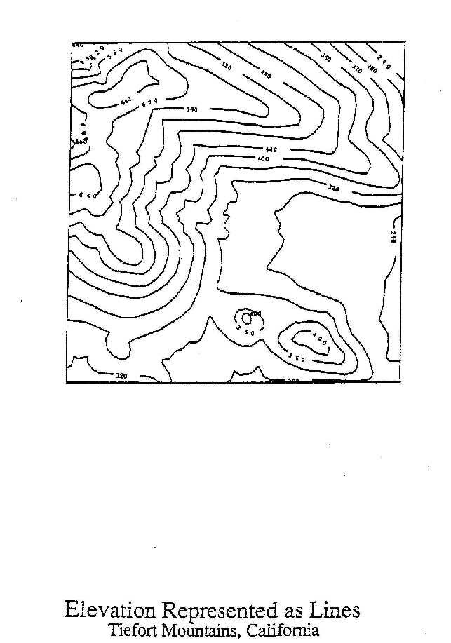
Other methods can be found in environmental modeling, but not commonly in GIS.
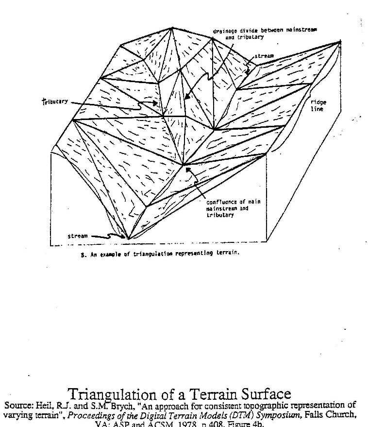
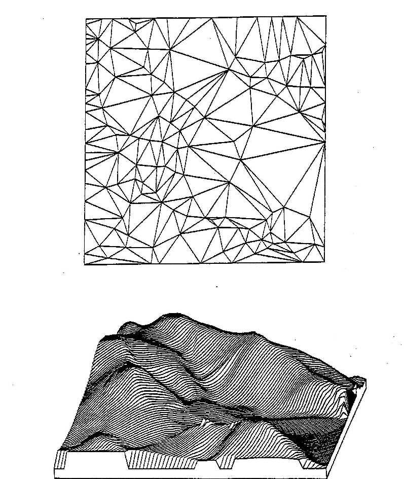
grid (a rectangular array of sample points) irregular points digitized contours polygons TIN finite element methods
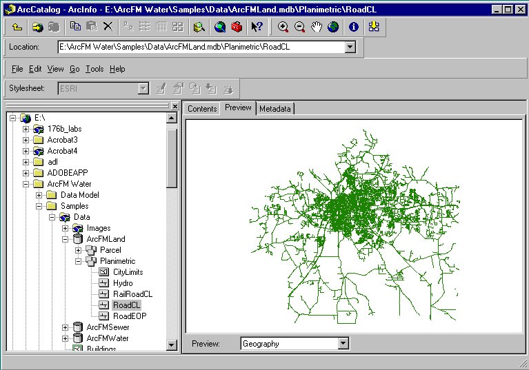
coveragebut not shapefiles in the Arc8 Geodatabase the distinction can be implemented in object behaviors
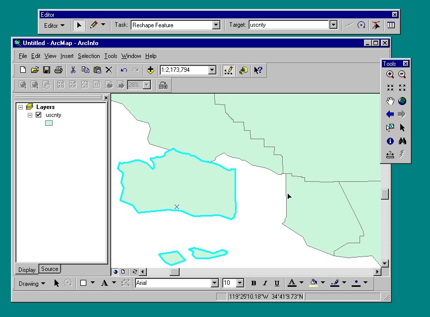
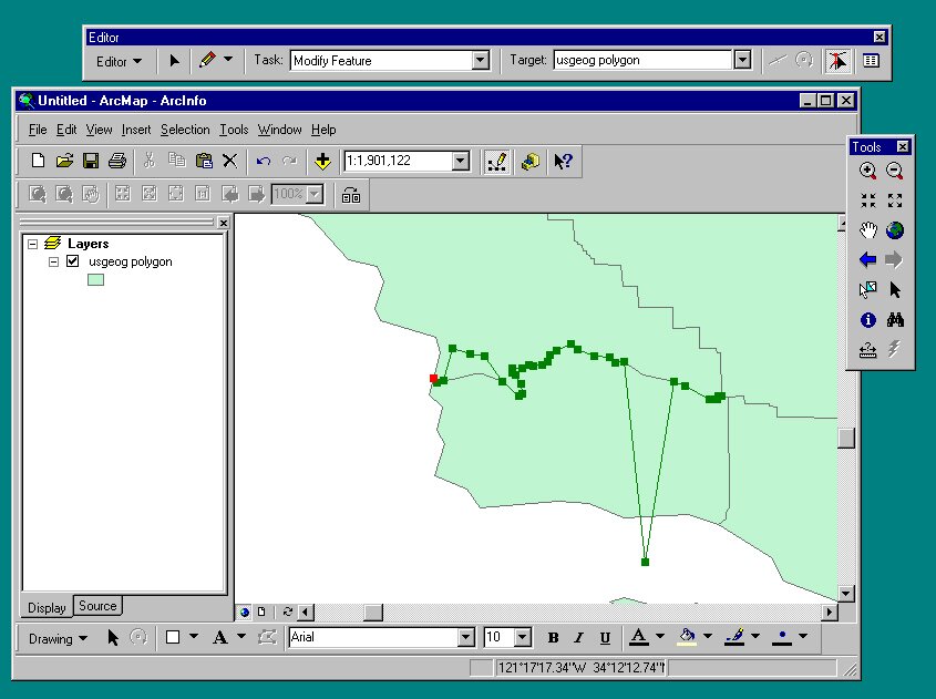
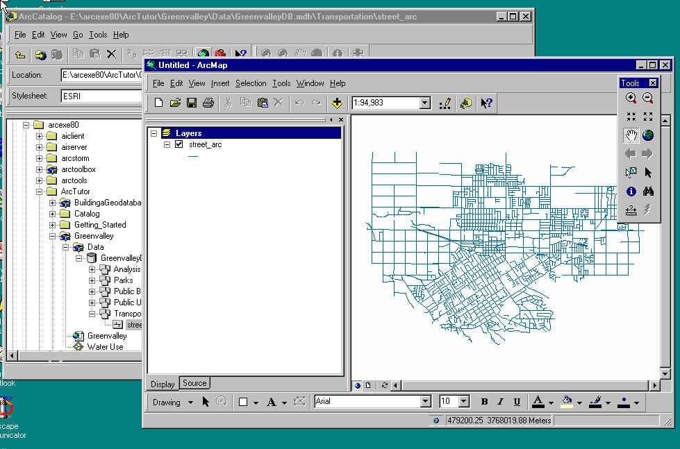
objects can be countedField and discrete object views can be implemented in either raster or vector formshow many mountains are there in Scotland?objects can be manipulated compare manipulation of shapefiles (objects) and coverages (fields) the distinction concerns how the world is conceived, and the rules governing object behaviorIf we ignore the field/discrete object distinction we may easily apply meaningless forms of analysis buffer makes sense only for discrete objects
numeric
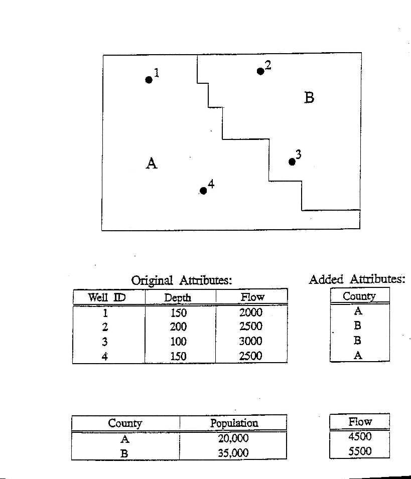
points (0-cells) A class of objects is a set with the same topological properties (e.g. all points) and with the same set of attributes (e.g. a set of wells or quarter sections or roads). In the Arc8 Geodatabase a class also has the same behaviors, and may inherit behaviors from other classes. A class is associated with an attribute table. Geodatabase introduces a consistent set of terms for primitive geometric objects
the layer provides one value at every point (recall the definition of a field)
Spatial objects are abstractions of reality. Some objects are well-defined (e.g. road, bridge) but others are not. Objects representing a discrete entity view tend to be well-defined; objects representing a field are not.
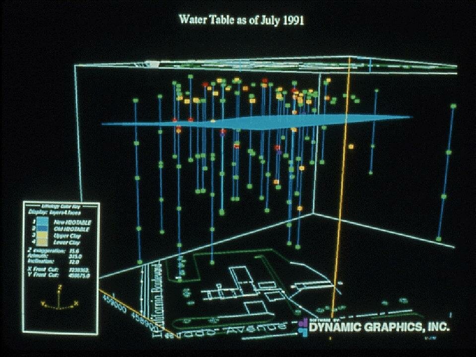
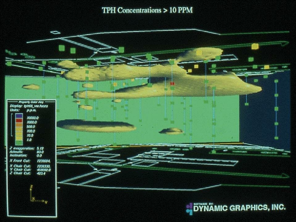
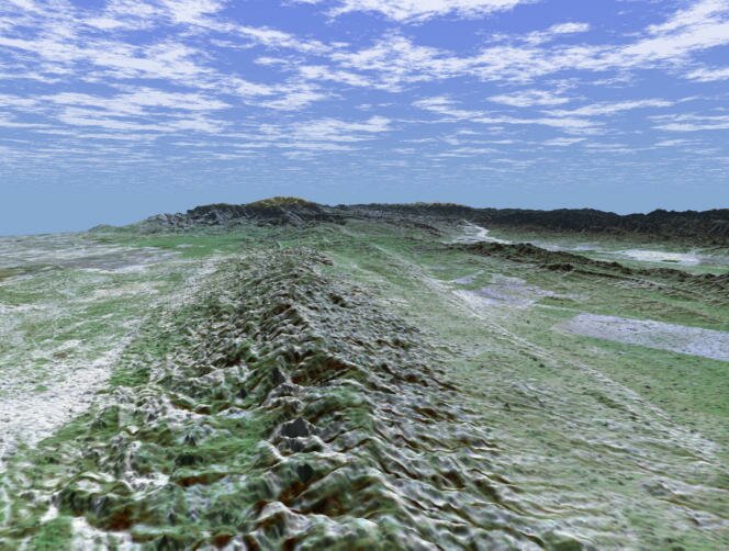
Slides: Elevation model options digital elevation model (raster)Advantages of TIN:
The methods used to store the attribute and locational information about the objects are not of immediate concern to the analyst/modeler.
A database encodes and represents the complex relationships which exist between objects.
Spatial relationships include:
The potential set of relationships within a complex spatial database is enormous. No system can afford to compute and store all of them in the database. A cartographic data structure stores no spatial relationships among objects.
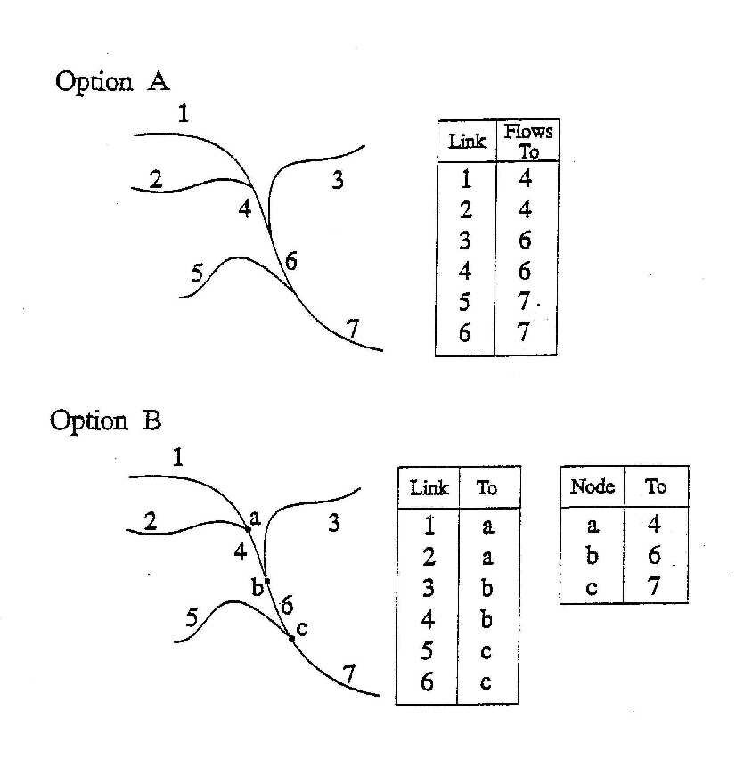
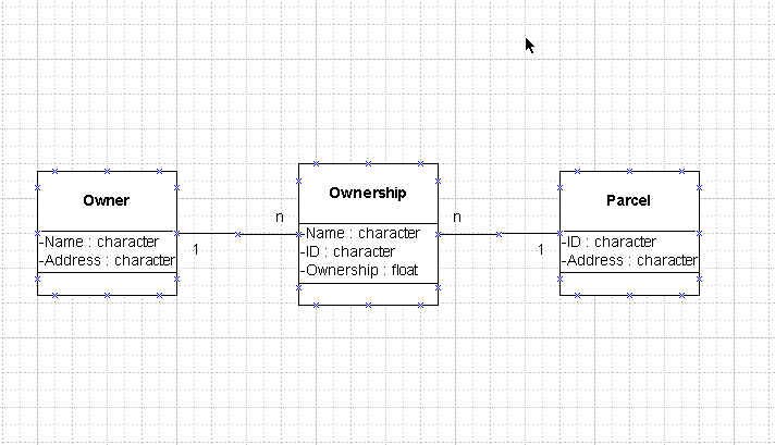
associationa functional linkage between objects in different classesaggregation and compositionlinkage between an object and its component objectstype inheritanceclasses inherit properties from more general classes An object pair is a combination of objects of the same or different types/classes which may have its own attributes.
giving attributes to associationsExamples of object pairs:
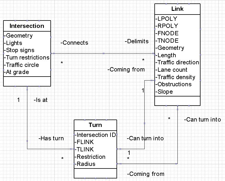
turntable (link-link pairs)
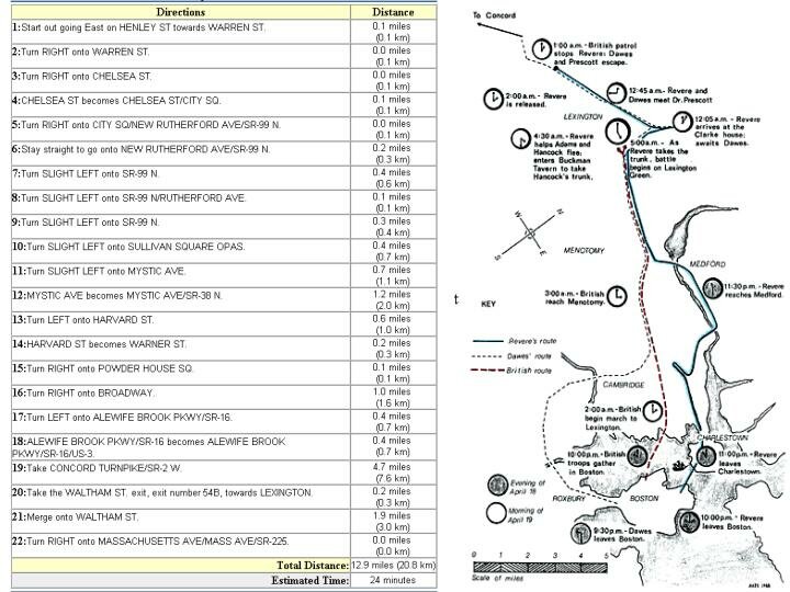
What are the essential components of a data model for route planning in a complex street network?
1. Design a database to capture and analyze data on recreational fishing in the Scottish Highlands, to support decision-making by the tourist industry and regulatory agencies. The database should be able to represent the following:
3. Design a database to support water resource analysis and planning for complex hydrographic networks that include streams, rivers, lakes and reservoirs. GEOGRAPHIC INFORMATION SYSTEM FUNCTION DESCRIPTIONS A. BASIC SYSTEM CAPABILITIES A1 Digitizing (di) Digitizing is the process of converting point and line data from source documents to a machine-readable format. A2 Edgematching (ed) Edgematching is the process of joining lines and polygons across map boundaries in creation of a "seamless" database.� The join should be topological as well as graphic, that is, a polygon so joined should become a single polygon in the data base, a line so joined should become a single line segment. A3 Polygonization (po) Polygonizing is the process of connecting together arcs ("spaghetti") to form polygons. A4 Labelling (la) This process transfers labels describing the contents (attributes) of polygons, and the characteristics of lines and points, to the digital system.� This input of labels must not be confused with the process of symbolizing and labelling output described below. A5 Reformatting digital data for input from other systems (rf) Data previously digitized are made accessible through an interface or converted by software to the system format, and made to be topologically useful as well as graphically compatible. A6 Reformatting for output to other systems (ro) This function is the inverse of the previous one. Internal data is reformatted to meet the requirements of other systems or standards. A7 Data base creation and management (db) Data is typically digitized from map-sheets, and may be edgematched. The creation of a true "seamless" database requires the establishment of a map sheet directory, and may include tiling to partition the database. A8 Raster/vector conversion (rv) The ability to convert data between vector and raster forms with grid cell size, position and orientation selected by the user. A9 Edit and display on input (ei) This function allows continuous display and editing of input data, usually in conjunction with digitizing. A10 Edit and display on output (eo) The ability to preview and edit displays before creation of hard copy maps. A11 Symbolizing (sy) To create high quality output from a GIS, it is necessary to be able to generate a wide variety of symbols to replace the primitive point, line and area objects stored in the database. A12 Plotting (pl) Creation of hard copy map output. A13 Updating (up) Updating of the digital data base with new points, lines, polygons and attributes. A14 Browsing (br) Browse is used to search the data base to answer simple locational queries, and includes pan and zoom. B. DATA MANIPULATION AND ANALYSIS FUNCTIONS B1 Create lists and reports (cl) This is the ability to create lists and reports on objects and their attributes in user-defined formats, and to include totals and subtotals. B2 Reclassify attributes (ra) Reclassification is the change in value of a set of existing attributes based on a set of user specified rules. B3 Dissolve lines and merge attributes (dm) Boundaries between adjacent polygons with identical attributes are dissolved to form larger polygons. B4 Line thinning and weeding (lt) This process is used to reduce the number of points defining a line or set of lines to a user defined tolerance. B5 Line smoothing (ls) Automatically smooth lines to a user-defined tolerance, creating a new set of points (compare B4). B6 Complex generalization (cg) Generalization which may require change in the type of an object, or relocation in response to cartographic rules. B7 Windowing (wi) The ability to clip features in the database to some defined polygon. B8 Centroid calculation and sequential numbering (cn) Calculate a contained, representative point in a polygon and assign a unique number to the new object. B9 Spot heights (sh) Given a digital elevation model, interpolate the height at any point. B10 Heights along streams (hs) Given a digital elevation model and a hydrology net, interpolate points along streams at fixed increments of height. B11 Contours (isolines) (ci) Given a set of regularly or irregularly spaced point values, interpolate contours at user-specified intervals. B12 Elevation polygons (ep) Given a digital elevation model, interpolate contours of height at user-specified intervals. B13 Watershed boundaries (wb) Given a digital elevation model and a hydrology net, interpolate the position of the watershed between basins. B14 Scale change (sc) Perform the operations associated with change of scale, which may include line thinning and generalization. B15 Rubber sheet stretching (rs) The ability to stretch one map image to fit over another, given common points of known locations. B16 Distortion elimination (de) The ability to remove various types of systematic distortion generated by different input methods. B17 Projection change (pc) The ability to transform maps from one map projection to another. B18 Generate points (gp) The ability to generate points and insert them in the database. B19 Generate lines (gl) The ability to generate lines and insert them in the database. B20 Generate polygons (ga) The ability to generate polygons and insert them in the database. B21 Generate circles (gc) The ability to generate circles defined by center point and radius. B22 Generate grid cell nets (gg) The ability to generate a network of grid cells given a point of origin, grid cell dimension and orientation. B23 Generate latitude/longitude nets (gn) The ability to generate graticules for a variety of map projections. B24 Generate corridors (gb) This process generates corridors of given width around existing points, lines or areas. B25 Generate graphs (gr) Create a graph illustrating attribute data by symbols, bars or fitted trend line. B26 Generate viewshed maps (gv) Given a digital elevation model and the locations of one or more viewpoints, generate polygons enclosing the area visible from at least one viewpoint. B27 Generate perspective views (ge) From a digital elevation model, generate a three-dimensional block diagram. B28 Generate cross sections (cs) Given a digital elevation model, show the cross-section along a user-specified line. B29 Search by attribute (sa) The ability to search the data base for objects with certain attributes. B30 Search by region (sr) The ability to search the data base within any region defined to the system. B31 Suppress (su) The ability to exclude objects by attribute (the converse of selecting by attribute). B32 Measure number of items (mi) The ability to count the number of objects in a class. B33 Measure distances along straight and convoluted lines (md) The ability to measure distances along a prescribed line. B34 Measure length of perimeter of areas (mp) The ability to measure the length of the perimeter of a polygon. B35 Measure size of areas (ma) The ability to measure the area of a polygon. B36 Measure volume (mv) The ability to compute the volume under a digital representation of a surface. B37 Calculate - arithmetic (ca) The ability to perform arithmetic, algebraic and Boolean calculations separately and in combination. B38 Calculate bearings between points (cb) The ability to calculate the bearing (with respect to True North) from a given point to another point. B39 Calculate vertical distance or height (ch) Given a digital elevation model, calculate the vertical distance (height) between two points. B40 Calculate slopes along lines (gradients) (al) The ability to measure the slope between two points of known height and location or to calculate the gradient between any two points along a convoluted line which contains two or more points of known elevation. B41 Calculate slopes of areas (sl) Given a digital elevation model and the boundary of a specified region (e.g., a part of a watershed), calculate the average slope of the region. B42 Calculate aspect of areas (aa) Given a digital elevation model and the boundary of a specified region, calculate the average aspect of the region. B43 Calculate angles and distances along linear features (ad) Given a prescribed linear feature, generalize its shape into a set of angles and distances from a start point, at user-set angular increments, and constrained to any known points along the linear feature. B44 Subdivide area according to a set of rules (sb) Given the corner points of a rectangular area, topologically subdivide the area into four quarters. B45 Locations from traverses (lo) Given a direction (one of eight radial directions) and distance from a given point, calculate the end point of the traverse. B46 Statistical functions (sf) The ability to carry out simple statistical analyses and tests on the database. B47 Graphic overlay (go) The ability to superimpose graphically one map on another and display the result on a screen or on a plot. B48 Point in polygon (pp) The ability to superimpose a set of points on a set of polygons and determine which polygon (if any) contains each point. B49 Line on polygon overlay (lp) The ability to superimpose a set of lines on a set of polygons, breaking the lines at intersections with polygon boundaries. B50 Polygon overlay (op) The ability to overlay digitally one set of polygons on another and form a topological intersection of the two, concatenating the attributes. B51 Sliver polygon removal (sp) The ability to delete automatically the small sliver polygons which result from a polygon overlay operation when certain polygon lines on the two maps represent different versions of the same physical line. B52 Line of sight (ln) The ability to determine the intervisibility of two points, or to determine those parts of pairs of lines or polygons which are intervisible. B53 Nearest neighbor search (nn) The ability to identify points, lines or polygons that are nearest to points, lines or polygons specified by location or attribute. B54 Shortest route (ps) The ability to determine the shortest or minimum cost route between two points or specified sets of points. B55 Contiguity analysis (co) The ability to identify areas that have a common boundary or node. B56 Connectivity analysis (cy) The ability to identify areas or points that are (or are not) connected to other areas or points by linear features. B57 Complex correlation (cx) The ability to compare maps representing different time periods, extracting differences or computing indices of change. B58 Weighted modelling (wm) The ability to assign weighting factors to individual data sets according to a set of rules and to overlay those data sets and carry out reclassify, dissolve and merge operations on the resulting concatenated data set. B59 Scene generation (sg) The ability to simulate an image of the appearance of an area from map data. The image would normally consist of an oblique view, with perspective. B60 Network analysis (na) Simple forms of network analysis are covered in Shortest route and Connectivity. More complex analyses are frequently carried out on network data by electrical and gas utilities, communications companies etc. These include the simulation of flows in complex networks, load balancing in electrical distribution, traffic analysis, and computation of pressure loss in gas pipes. In many cases these capabilities can be found in existing packages which can be interfaced to the GIS database. Other groupings of GIS functions: Berry, J.K., 1987, "Fundamental operations in computer-assisted map analysis". International Journal of GIS 1 119-36.
Tomlin, Dana, 1990. Geographic Information Systems and Cartographic Modeling. Prentice Hall.
1. Query and reasoning based on database viewscatalog
simple geometric measurements associated with objects3. Transformationarea, distance, length, perimeter, shape buffers4. Descriptive summaries centers5. Optimization best routes6. Hypothesis testingraster versionbest locations inference from sample to population Integration of GIS and Spatial Analysis 1. Full integration (embedding)
|